Aerospace Design via Quasiconvex Optimization

Consider a triangle, or a wedge, located within a hypersonic flow. A standard aerospace design optimization problem is to design the wedge to maximize the lift-to-drag ratio (L/D) (or conversely minimize the D/L ratio), subject to certain geometric constraints. In this example, the wedge is known to have a constant hypotenuse, and our job is to choose its width and height.

The drag-to-lift ratio is given by

\[\frac{\mathrm{D}}{\mathrm{L}} = \frac{\mathrm{c_d}}{\mathrm{c_l}},\]

where \(\mathrm{c_d}\) and \(\mathrm{c_l}\) are drag and lift coefficients, respectively, that are obtained by integrating the projection of the pressure coefficient in directions parallel to, and perpendicular to, the body.

It turns out that the the drag-to-lift ratio is a quasilinear function, as we’ll now show. We will assume the pressure coefficient is given by the Newtonian sine-squared law for whetted areas of the body,

\[\mathrm{c_p} = 2(\hat{v}\cdot\hat{n})^2\]

and elsewhere \(\mathrm{c_p} = 0\). Here, \(\hat{v}\) is the free stream direction, which for simplicity we will assume is parallel to the body so that, \(\hat{v} = \langle 1, 0 \rangle\), and \(\hat{n}\) is the local unit normal. For a wedge defined by width \(\Delta x\), and height \(\Delta y\),

\[\hat{n} = \langle -\Delta y/s,-\Delta x/s \rangle\]

where \(s\) is the hypotenuse length. Therefore,

\[\mathrm{c_p} = 2((1)(-\Delta y/s)+(0)(-\Delta x/s))^2 = \frac{2 \Delta y^2}{s^2}\]

The lift and drag coefficients are given by

\[\begin{split}\begin{align*} \mathrm{c_d} &= \frac{1}{c}\int_0^s -\mathrm{c_p}\hat{n}_x \mathrm{d}s \\ \mathrm{c_l} &= \frac{1}{c}\int_0^s -\mathrm{c_p}\hat{n}_y \mathrm{d}s \end{align*}\end{split}\]

Where \(c\) is the reference chord length of the body. Given that \(\hat{n}\), and therefore \(\mathrm{c_p}\) are constant over the whetted surface of the body,

\[\begin{split}\begin{align*} \mathrm{c_d} &= -\frac{s}{c}\mathrm{c_p}\hat{n}_x = \frac{s}{c}\frac{2 \Delta y^2}{s^2}\frac{\Delta y}{s} \\ \mathrm{c_l} &= -\frac{s}{c}\mathrm{c_p}\hat{n}_y = \frac{s}{c}\frac{2 \Delta y^2}{s^2}\frac{\Delta x}{s} \end{align*}\end{split}\]

Assuming \(s=1\), so that \(\Delta y = \sqrt{1-\Delta x^2}\), plugging in the above into the equation for \(D/L\), we obtain

\[\frac{\mathrm{D}}{\mathrm{L}} = \frac{\Delta y}{\Delta x} = \frac{\sqrt{1-\Delta x^2}}{\Delta x} = \sqrt{\frac{1}{\Delta x^2}-1}.\]

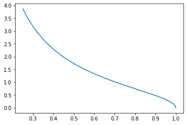
This function is representable as a DQCP, quasilinear function. We plot it below, and then we write it using DQCP.

%matplotlib inline

import matplotlib
import numpy as np
import matplotlib.pyplot as plt
import math

x = np.linspace(.25,1,num=201)
obj = []
for i in range(len(x)):
    obj.append(math.sqrt(1/x[i]**2-1))

plt.plot(x,obj)

[<matplotlib.lines.Line2D at 0x7f571d7bfdd8>]

import cvxpy as cp

x = cp.Variable(pos=True)
obj = cp.sqrt(cp.inv_pos(cp.square(x))-1)
print("This objective function is", obj.curvature)

This objective function is QUASILINEAR

Minimizing this objective function subject to constraints representing payload requirements is a standard aerospace design problem. In this case we will consider the constraint that the wedge must be able to contain a rectangle of given length and width internally along its hypotenuse. This is representable as a convex constraint.

a = .05 # USER INPUT: height of rectangle, should be at most b
b = .65 # USER INPUT: width of rectangle
constraint = [a*cp.inv_pos(x)-(1-b)*cp.sqrt(1-cp.square(x))<=0]
print(constraint)

[Inequality(Expression(CONVEX, UNKNOWN, ()))]

prob = cp.Problem(cp.Minimize(obj), constraint)
prob.solve(qcp=True, verbose=True)
print('Final L/D Ratio = ', 1/obj.value)
print('Final width of wedge = ', x.value)
print('Final height of wedge = ', math.sqrt(1-x.value**2))

****************************************************************************
Preparing to bisect problem

minimize 0.0
subject to 0.05 * var30766 + -0.35 * var30793 <= 0.0
           SOC(reshape(var30747 + var30766, (1,)), Vstack(reshape(var30747 + -var30766, (1, 1)), reshape(2.0 * 1.0, (1, 1))))
           SOC(reshape(var30779 + 1.0, (1,)), Vstack(reshape(var30779 + -1.0, (1, 1)), reshape(2.0 * var30747, (1, 1))))
           SOC(reshape(1.0 + -var30779 + 1.0, (1,)), Vstack(reshape(1.0 + -var30779 + -1.0, (1, 1)), reshape(2.0 * var30793, (1, 1))))
           power(power(power(param30811, 2) + --1.0, -1), 1/2) <= var30747

Finding interval for bisection ...
initial lower bound: 0.000000
initial upper bound: 1.000000

(iteration 0) lower bound: 0.000000
(iteration 0) upper bound: 1.000000
(iteration 0) query point: 0.500000
(iteration 0) query was feasible. Solution(status=optimal, opt_val=0.0, primal_vars={30766: array(1.28425055), 30793: array(0.32048066), 30747: 0.9203698369509382, 30779: array(0.86287821)}, dual_vars={30764: 1.184352986830617e-10, 30775: array([ 7.68139086e-12, -9.11799720e-13, -6.85059567e-12]), 30788: array([ 6.73308751e-11,  7.50722737e-12, -6.55220021e-11]), 30802: array([ 4.04979217e-11,  3.43109122e-11, -1.68754271e-11]), 30835: 1.4165742899966837e-10}, attr={'solve_time': 6.0109e-05, 'setup_time': 4.4997e-05, 'num_iters': 7}))

(iteration 5) lower bound: 0.125000
(iteration 5) upper bound: 0.156250
(iteration 5) query point: 0.140625
(iteration 5) query was infeasible.

(iteration 10) lower bound: 0.145508
(iteration 10) upper bound: 0.146484
(iteration 10) query point: 0.145996
(iteration 10) query was feasible. Solution(status=optimal, opt_val=0.0, primal_vars={30766: array(1.01067238), 30793: array(0.14440604), 30747: 0.9895144829793, 30779: array(0.97914383)}, dual_vars={30764: 1.2610785752467482e-05, 30775: array([ 6.37367039e-07,  6.73702792e-09, -6.37322961e-07]), 30788: array([ 1.50627898e-05,  1.58286953e-07, -1.50619494e-05]), 30802: array([ 7.77053008e-06,  7.45051237e-06, -2.20683981e-06]), 30835: 2.948014872712083e-05}, attr={'solve_time': 0.000114922, 'setup_time': 3.6457e-05, 'num_iters': 10}))

(iteration 15) lower bound: 0.145874
(iteration 15) upper bound: 0.145905
(iteration 15) query point: 0.145889
(iteration 15) query was infeasible.

Bisection completed, with lower bound 0.145897 and upper bound 0.1458979
****************************************************************************

Final L/D Ratio =  6.854107648695203
Final width of wedge =  0.9895238539767502
Final height of wedge =  0.14436946495363565

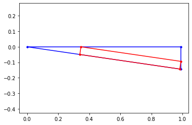
Once the solution has been found, we can create a plot to verify that the rectangle is inscribed within the wedge.

y = math.sqrt(1-x.value**2)
lambda1 = a*x.value/y
lambda2 = a*x.value**2/y+a*y
lambda3 = a*x.value-y*(a*x.value/y-b)

plt.plot([0,x.value],[0,0],'b.-')
plt.plot([0,x.value],[0,-y],'b.-')
plt.plot([x.value,x.value],[0,-y],'b.-')

pt1 = [lambda1*x.value,-lambda1*y]
pt2 = [(lambda1+b)*x.value,-(lambda1+b)*y]
pt3 = [(lambda1+b)*x.value+a*y,-(lambda1+b)*y+a*x.value]
pt4 = [lambda1*x.value+a*y,-lambda1*y+a*x.value]

plt.plot([pt1[0],pt2[0]],[pt1[1],pt2[1]],'r.-')
plt.plot([pt2[0],pt3[0]],[pt2[1],pt3[1]],'r.-')
plt.plot([pt3[0],pt4[0]],[pt3[1],pt4[1]],'r.-')
plt.plot([pt4[0],pt1[0]],[pt4[1],pt1[1]],'r.-')

plt.axis('equal')

(-0.04947620645689951,
 1.0390003355948896,
 -0.15158793820131744,
 0.0072184732476817896)