Sparse signal recovery¶

This example is adapted from Cederberg, Zhang, Nobel, and Boyd, “Disciplined Nonlinear Programming“.

In this example, the goal is to recover a sparse signal \(x_0 \in \mathbf{R}^n\) from a given measurement vector \(y = Ax_0\), where \(A \in \mathbf{R}^{m \times n}\) (with \(m < n\)) is a known sensing matrix [26]. A common heuristic based on convex optimization is to minimize the \(\ell_1\) norm of \(x\) subject to \(Ax = y\). An alternative approach based on nonconvex optimization is to minimize the sum of the square roots of the absolute values of the entries of \(x\), which tends to promote sparsity more aggressively. This leads to the problem

\[\begin{split}\begin{array}{ll} \mbox{minimize} & \sum_{i=1}^{n} \sqrt{|x_i|} \\ \mbox{subject to} & Ax = y, \end{array}\end{split}\]

with variable \(x\). This problem is DNLP-compliant since the objective is L-convex.

DNLP specification. The code specifying this problem is given below. For this example, we use Knitro’s interior-point method as the solver, because Ipopt failed to solve this problem reliably. The issue likely arises from the fact that the objective function gradient becomes infinite as any entry of x approaches zero, so no KKT point exists for the canonicalized problem.

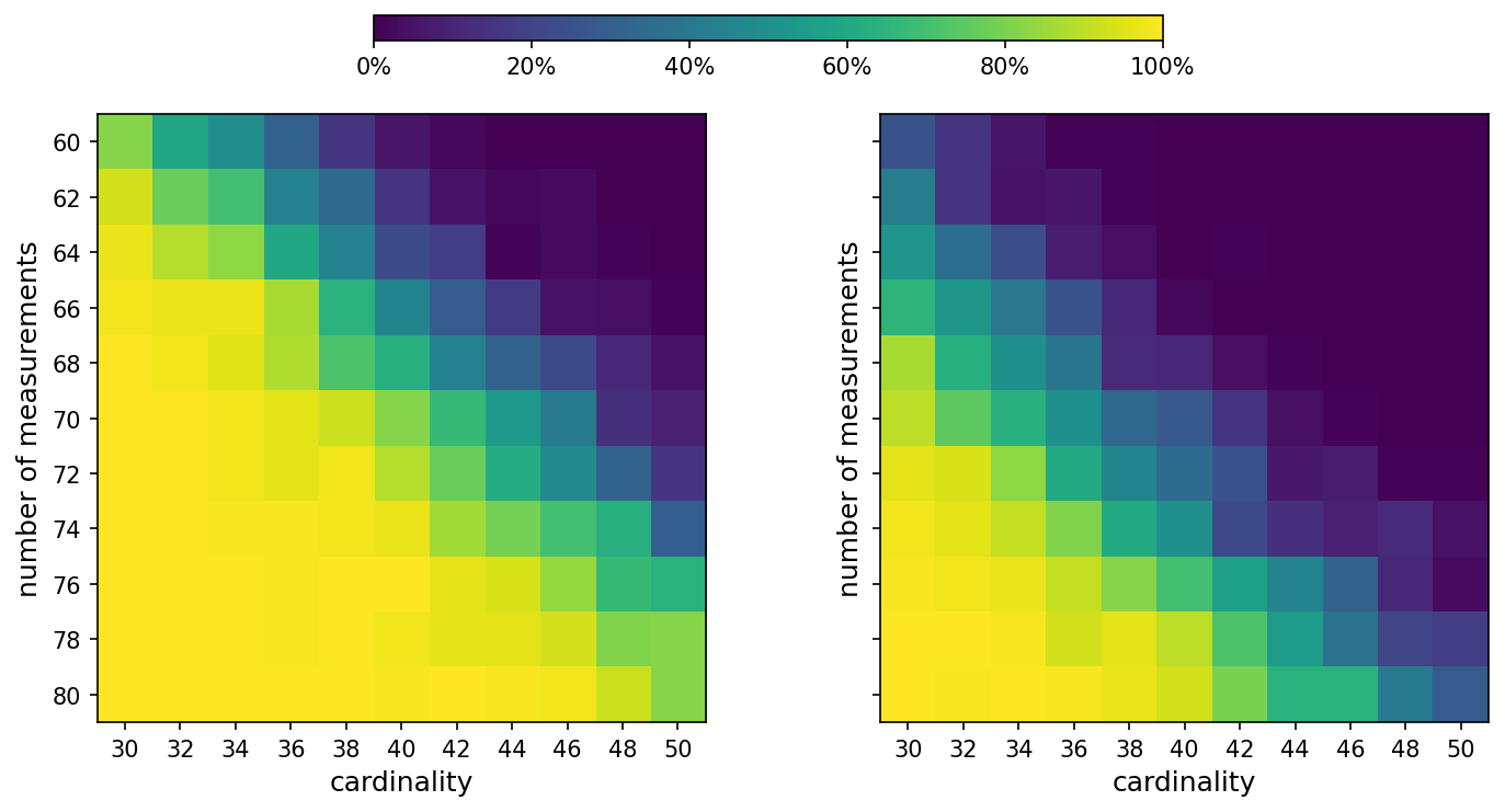
We consider a simulation with signal dimension n = 100, where we vary the number of measurements m from 60 to 80, and the cardinality of the true signal \(x_0\) from 30 to 50. The positions of the nonzero entries of \(x_0\) are sampled from a uniform distribution, with the nonzero values chosen as \(\mathcal{N}(0, 25)\) random variables. The entries of A are sampled from a standard normal distribution. We say that the recovery is successful if the relative error \(\|\hat{x} - x_0\|_2 / \|x_0\|_2\) is less than \(10^{-2}\), where \(\hat{x}\) is the recovered signal. To estimate the probability of successful recovery for each pair of number of measurements and signal cardinality, we repeat the simulation 100 times and compute the fraction of successful recoveries.

import matplotlib.pyplot as plt
import numpy as np
import numpy.linalg as LA
import cvxpy as cp
from matplotlib.ticker import PercentFormatter

rng = np.random.default_rng(0)
n, T = 100, 100
m = list(range(60, 81, 2))
k = list(range(30, 51, 2))

RECOVERY_TOL = 1e-2
probabilities_noncvx = np.zeros((len(m), len(k)))
probabilities_cvx = np.zeros((len(m), len(k)))

for time in range(T):
   print(f"Trial {time+1} of {T}")
   for kk in k:
      x0 = np.zeros((n,))
      ind = rng.permutation(n)
      ind = ind[0:kk]
      x0[ind] = rng.standard_normal((kk,)) * 5

      for mm in m:
            A = rng.standard_normal((mm, n))
            y = A @ x0

            # nonconvex recovery
            x = cp.Variable((n, ))
            prob = cp.Problem(cp.Minimize(cp.sum(cp.sqrt(cp.abs(x)))), [A @ x == y])
            prob.solve(nlp=True, solver=cp.KNITRO, verbose=False, algorithm=1)
            x_noncvx_recovery = x.value

            # convex recovery
            x = cp.Variable((n, ))
            prob = cp.Problem(cp.Minimize(cp.norm1(x)), [A @ x == y])
            prob.solve(solver=cp.CLARABEL)
            x_cvx_recovery = x.value

            # were the recoveries successful?
            noncvx_success = LA.norm(x_noncvx_recovery - x0, 2) / LA.norm(x0, 2) <= RECOVERY_TOL
            cvx_success = LA.norm(x_cvx_recovery - x0, 2) / LA.norm(x0, 2) <= RECOVERY_TOL
            probabilities_noncvx[m.index(mm), k.index(kk)] += int(noncvx_success)
            probabilities_cvx[m.index(mm), k.index(kk)] += int(cvx_success)

probabilities_cvx /= T
probabilities_noncvx /= T

We see below that the nonconvex approach is more has a higher probability of recovery than the convex approach. Left: Approach based on nonconvex optimization. Right: Approach based on convex optimization.

fig, axes = plt.subplots(1, 2, figsize=(12, 5), dpi=150, sharey=True,
                      gridspec_kw={'wspace': 0.05})

im1 = axes[0].imshow(probabilities_noncvx, interpolation="none")
axes[0].set_xticks(range(len(k))); axes[0].set_xticklabels(k)
axes[0].set_yticks(range(len(m))); axes[0].set_yticklabels(m)
axes[0].set_xlabel("cardinality", fontsize=12)
axes[0].set_ylabel("number of measurements", fontsize=12)

im2 = axes[1].imshow(probabilities_cvx, interpolation="none")
axes[1].set_xticks(range(len(k))); axes[1].set_xticklabels(k)
axes[1].set_yticks(range(len(m))); axes[1].set_yticklabels(m)
axes[1].set_xlabel("cardinality", fontsize=12)
axes[1].set_ylabel("number of measurements", fontsize=12)

# Shared colorbar on top
# Shared colorbar placed in a fixed figure slot (doesn't change subplot sizes)
cax = fig.add_axes([0.3, 0.94, 0.4, 0.03])  # [left, bottom, width, height] in figure coords
cbar = fig.colorbar(im1, cax=cax, orientation='horizontal')
cbar.ax.xaxis.set_major_formatter(PercentFormatter(xmax=1.0))
fig.subplots_adjust(top=0.85)