Structured prediction

In this example\(\newcommand{\reals}{\mathbf{R}}\)\(\newcommand{\ones}{\mathbf{1}}\), we fit a regression model to structured data, using an LLCP. The training dataset \(\mathcal D\) contains \(N\) input-output pairs \((x, y)\), where \(x \in \reals^{n}_{++}\) is an input and \(y \in \reals^{m}_{++}\) is an outputs. The entries of each output \(y\) are sorted in ascending order, meaning \(y_1 \leq y_2 \leq \cdots \leq y_m\).

Our regression model \(\phi : \reals^{n}_{++} \to \reals^{m}_{++}\) takes as input a vector \(x \in \reals^{n}_{++}\), and solves an LLCP to produce a prediction \(\hat y \in \reals^{m}_{++}\). In particular, the solution of the LLCP is model’s prediction. The model is of the form

\[\begin{split}\begin{equation} \begin{array}{lll} \phi(x) = & \mbox{argmin} & \ones^T (z/y + y / z) \\ & \mbox{subject to} & y_i \leq y_{i+1}, \quad i=1, \ldots, m-1 \\ && z_i = c_i x_1^{A_{i1}}x_2^{A_{i2}}\cdots x_n^{A_{in}}, \quad i = 1, \ldots, m. \end{array}\label{e-model} \end{equation}\end{split}\]

Here, the minimization is over \(y \in \reals^{m}_{++}\) and an auxiliary variable \(z \in \reals^{m}_{++}\), \(\phi(x)\) is the optimal value of \(y\), and the parameters are \(c \in \reals^{m}_{++}\) and \(A \in \reals^{m \times n}\). The ratios in the objective are meant elementwise, as is the inequality \(y \leq z\), and \(\ones\) denotes the vector of all ones. Given a vector \(x\), this model finds a sorted vector \(\hat y\) whose entries are close to monomial functions of \(x\) (which are the entries of \(z\)), as measured by the fractional error.

The training loss \(\mathcal{L}(\phi)\) of the model on the training set is the mean squared loss

\[\mathcal{L}(\phi) = \frac{1}{N}\sum_{(x, y) \in \mathcal D} \|y - \phi(x)\|_2^2.\]

We emphasize that \(\mathcal{L}(\phi)\) depends on \(c\) and \(A\). In this example, we fit the parameters \(c\) and \(A\) in the LLCP to minimize the training loss \(\mathcal{L}(\phi)\).

Fitting. We fit the parameters by an iterative projected gradient descent method on \(\mathcal L(\phi)\). In each iteration, we first compute predictions \(\phi(x)\) for each input in the training set; this requires solving \(N\) LLCPs. Next, we evaluate the training loss \(\mathcal L(\phi)\). To update the parameters, we compute the gradient \(\nabla \mathcal L(\phi)\) of the training loss with respect to the parameters \(c\) and \(A\). This requires differentiating through the solution map of the LLCP. We can compute this gradient efficiently, using the backward method in CVXPY (or CVXPY Layers). Finally, we subtract a small multiple of the gradient from the parameters. Care must be taken to ensure that \(c\) is strictly positive; this can be done by clamping the entries of \(c\) at some small threshold slightly above zero. We run this method for a fixed number of iterations.

This example is described in the paper Differentiating through Log-Log Convex Programs.

Shane Barratt formulated the idea of using an optimization layer to regress on sorted vectors.

Requirements. This example requires PyTorch and CvxpyLayers >= v0.1.3.

from cvxpylayers.torch import CvxpyLayer


import cvxpy as cp
import matplotlib.pyplot as plt
import numpy as np
import torch

torch.set_default_tensor_type(torch.DoubleTensor)
%matplotlib inline

Data generation

n = 20
m = 10

# Number of training input-output pairs
N = 100

# Number of validation pairs
N_val = 50

torch.random.manual_seed(243)
np.random.seed(243)

normal = torch.distributions.multivariate_normal.MultivariateNormal(torch.zeros(n), torch.eye(n))
lognormal = lambda batch: torch.exp(normal.sample(torch.tensor([batch])))

A_true = torch.randn((m, n)) / 10
c_true = np.abs(torch.randn(m))

def generate_data(num_points, seed):
    torch.random.manual_seed(seed)
    np.random.seed(seed)

    latent = lognormal(num_points)
    noise = lognormal(num_points)
    inputs = noise + latent

    input_cp = cp.Parameter(pos=True, shape=(n,))
    prediction = cp.multiply(c_true.numpy(), cp.gmatmul(A_true.numpy(), input_cp))
    y = cp.Variable(pos=True, shape=(m,))
    objective_fn = cp.sum(prediction / y + y/prediction)
    constraints = []
    for i in range(m-1):
        constraints += [y[i] <= y[i+1]]
    problem = cp.Problem(cp.Minimize(objective_fn), constraints)

    outputs = []
    for i in range(num_points):
        input_cp.value = inputs[i, :].numpy()
        problem.solve(cp.SCS, gp=True)
        outputs.append(y.value)
    return inputs, torch.stack([torch.tensor(t) for t in outputs])

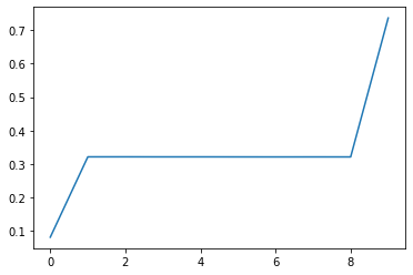
train_inputs, train_outputs = generate_data(N, 243)
plt.plot(train_outputs[0, :].numpy())

[<matplotlib.lines.Line2D at 0x12b367cd0>]

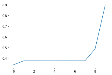
val_inputs, val_outputs = generate_data(N_val, 0)
plt.plot(val_outputs[0, :].numpy())

[<matplotlib.lines.Line2D at 0x12da7e410>]

Monomial fit to each component

We will initialize the parameters in our LLCP model by fitting monomials to the training data, without enforcing the monotonicity constraint.

log_c = cp.Variable(shape=(m,1))
theta = cp.Variable(shape=(n, m))
inputs_np = train_inputs.numpy()
log_outputs_np = np.log(train_outputs.numpy()).T
log_inputs_np = np.log(inputs_np).T
offsets = cp.hstack([log_c]*N)

cp_preds = theta.T @ log_inputs_np + offsets
objective_fn = (1/N) * cp.sum_squares(cp_preds - log_outputs_np)
lstq_problem = cp.Problem(cp.Minimize(objective_fn))

lstq_problem.is_dcp()

True

lstq_problem.solve(verbose=True)

-----------------------------------------------------------------
           OSQP v0.6.0  -  Operator Splitting QP Solver
              (c) Bartolomeo Stellato,  Goran Banjac
        University of Oxford  -  Stanford University 2019
-----------------------------------------------------------------
problem:  variables n = 1210, constraints m = 1000
          nnz(P) + nnz(A) = 23000
settings: linear system solver = qdldl,
          eps_abs = 1.0e-05, eps_rel = 1.0e-05,
          eps_prim_inf = 1.0e-04, eps_dual_inf = 1.0e-04,
          rho = 1.00e-01 (adaptive),
          sigma = 1.00e-06, alpha = 1.60, max_iter = 10000
          check_termination: on (interval 25),
          scaling: on, scaled_termination: off
          warm start: on, polish: on, time_limit: off

iter   objective    pri res    dua res    rho        time
   1   0.0000e+00   3.30e+00   1.22e+04   1.00e-01   3.06e-03s
  50   1.0014e-02   1.72e-07   1.64e-07   1.75e-03   7.37e-03s
plsh   1.0014e-02   1.56e-15   1.17e-14   --------   9.68e-03s

status:               solved
solution polish:      successful
number of iterations: 50
optimal objective:    0.0100
run time:             9.68e-03s
optimal rho estimate: 8.77e-05

0.010014212812318733

c = torch.exp(torch.tensor(log_c.value)).squeeze()
lstsq_val_preds = []
for i in range(N_val):
    inp = val_inputs[i, :].numpy()
    pred = cp.multiply(c,cp.gmatmul(theta.T.value, inp))
    lstsq_val_preds.append(pred.value)

Fitting

A_param = cp.Parameter(shape=(m, n))
c_param = cp.Parameter(pos=True, shape=(m,))
x_slack = cp.Variable(pos=True, shape=(n,))
x_param = cp.Parameter(pos=True, shape=(n,))
y = cp.Variable(pos=True, shape=(m,))

prediction = cp.multiply(c_param, cp.gmatmul(A_param, x_slack))
objective_fn = cp.sum(prediction / y + y / prediction)
constraints = [x_slack == x_param]
for i in range(m-1):
    constraints += [y[i] <= y[i+1]]
problem = cp.Problem(cp.Minimize(objective_fn), constraints)
problem.is_dgp(dpp=True)

True

A_param.value = np.random.randn(m, n)
x_param.value = np.abs(np.random.randn(n))
c_param.value = np.abs(np.random.randn(m))

layer = CvxpyLayer(problem, parameters=[A_param, c_param, x_param], variables=[y], gp=True)

torch.random.manual_seed(1)
A_tch = torch.tensor(theta.T.value)
A_tch.requires_grad_(True)
c_tch = torch.tensor(np.squeeze(np.exp(log_c.value)))
c_tch.requires_grad_(True)
train_losses = []
val_losses = []

lam1 = torch.tensor(1e-1)
lam2 = torch.tensor(1e-1)

opt = torch.optim.SGD([A_tch, c_tch], lr=5e-2)
for epoch in range(10):
    preds = layer(A_tch, c_tch, train_inputs, solver_args={'acceleration_lookback': 0})[0]
    loss = (preds - train_outputs).pow(2).sum(axis=1).mean(axis=0)

    with torch.no_grad():
        val_preds = layer(A_tch, c_tch, val_inputs, solver_args={'acceleration_lookback': 0})[0]
        val_loss = (val_preds - val_outputs).pow(2).sum(axis=1).mean(axis=0)

    print('(epoch {0}) train / val ({1:.4f} / {2:.4f}) '.format(epoch, loss, val_loss))
    train_losses.append(loss.item())
    val_losses.append(val_loss.item())

    opt.zero_grad()
    loss.backward()
    opt.step()
    with torch.no_grad():
        c_tch = torch.max(c_tch, torch.tensor(1e-8))

(epoch 0) train / val (0.0018 / 0.0014)
(epoch 1) train / val (0.0017 / 0.0014)
(epoch 2) train / val (0.0017 / 0.0014)
(epoch 3) train / val (0.0017 / 0.0014)
(epoch 4) train / val (0.0017 / 0.0014)
(epoch 5) train / val (0.0017 / 0.0014)
(epoch 6) train / val (0.0016 / 0.0014)
(epoch 7) train / val (0.0016 / 0.0014)
(epoch 8) train / val (0.0016 / 0.0014)
(epoch 9) train / val (0.0016 / 0.0014)

with torch.no_grad():
    train_preds_tch = layer(A_tch, c_tch, train_inputs)[0]
    train_preds = [t.detach().numpy() for t in train_preds_tch]

with torch.no_grad():
    val_preds_tch = layer(A_tch, c_tch, val_inputs)[0]
    val_preds = [t.detach().numpy() for t in val_preds_tch]

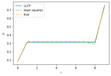
fig = plt.figure()


i = 0
plt.plot(val_preds[i], label='LLCP', color='teal')
plt.plot(lstsq_val_preds[i], label='least squares', linestyle='--', color='gray')
plt.plot(val_outputs[i], label='true', linestyle='-.', color='orange')
w, h = 8, 3.5
plt.xlabel(r'$i$')
plt.ylabel(r'$y_i$')
plt.legend()
plt.show()