Sparse covariance estimation for Gaussian variables
A derivative work by Judson Wilson, 5/22/2014. Adapted (with significant improvements and fixes) from the CVX example of the same name, by Joelle Skaf, 4/24/2008.
Topic References:
Section 7.1.1, Boyd & Vandenberghe “Convex Optimization”
Introduction
Suppose \(y \in \mathbf{\mbox{R}}^n\) is a Gaussian random variable with zero mean and covariance matrix \(R = \mathbf{\mbox{E}}[yy^T]\), with sparse inverse \(S = R^{-1}\) (\(S_{ij} = 0\) means that \(y_i\) and \(y_j\) are conditionally independent). We want to estimate the covariance matrix \(R\) based on \(N\) independent samples \(y_1,\dots,y_N\) drawn from the distribution, and using prior knowledge that \(S\) is sparse
A good heuristic for estimating \(R\) is to solve the problem
where \(Y\) is the sample covariance of \(y_1,\dots,y_N\), and \(\alpha\) is a sparsity parameter to be chosen or tuned.
Generate problem data
import cvxpy as cp
import numpy as np
import scipy as scipy

# Fix random number generator so we can repeat the experiment.
np.random.seed(0)

# Dimension of matrix.
n = 10

# Number of samples, y_i
N = 1000

# Create sparse, symmetric PSD matrix S
A = np.random.randn(n, n)  # Unit normal gaussian distribution.
A[scipy.sparse.random_array((n, n), density=0.85).todense().nonzero()] = 0  # Sparsen A
Strue = A.dot(A.T) + 0.05 * np.eye(n)  # Force strict pos. def.

# Create the covariance matrix associated with S.
R = np.linalg.inv(Strue)

# Create samples y_i from the distribution with covariance R.
y_sample = scipy.linalg.sqrtm(R).dot(np.random.randn(n, N))

# Calculate the sample covariance matrix.
Y = np.cov(y_sample)
Solve for several \(\alpha\) values
# The alpha values for each attempt at generating a sparse inverse cov. matrix.
alphas = [10, 2, 1]

# Empty list of result matrixes S
Ss = []

# Solve the optimization problem for each value of alpha.
for alpha in alphas:
    # Create a variable that is constrained to the positive semidefinite cone.
    S = cp.Variable(shape=(n,n), PSD=True)

    # Form the logdet(S) - tr(SY) objective.
    # Use vdot(S, Y) as alternate formulation for trace(S@Y)
    # trace(S@Y) only requires diagonal entries of S@Y, which can be
    # computed by taking the sum of the element-wise product of S.T and Y in O(n^2) time.
    # vdot does this operation directly.
    obj = cp.Maximize(cp.log_det(S) - cp.vdot(S, Y))

    # Set constraint.
    constraints = [cp.sum(cp.abs(S)) <= alpha]

    # Form and solve optimization problem.
    prob = cp.Problem(obj, constraints)
    prob.solve(solver=cp.CVXOPT)
    if prob.status != cp.OPTIMAL:
        raise Exception('CVXPY Error')

    # If the covariance matrix R is desired, here is how to create it.
    R_hat = np.linalg.inv(S.value)

    # Threshold S element values to enforce exact zeros:
    S = S.value
    S[abs(S) <= 1e-4] = 0

    # Store this S in the list of results for later plotting.
    Ss += [S]

    print('Completed optimization parameterized by alpha = {}, obj value = {}'.format(alpha, obj.value))
Completed optimization parameterized by alpha = 10, obj value = -16.167608186713004
Completed optimization parameterized by alpha = 2, obj value = -22.545759632606043
Completed optimization parameterized by alpha = 1, obj value = -26.989407069609157
Result plots
import matplotlib.pyplot as plt
# Show plot inline in ipython.
%matplotlib inline
# Plot properties.
plt.rc('text', usetex=True)
plt.rc('font', family='serif')
# Create figure.
plt.figure()
plt.figure(figsize=(12, 12))
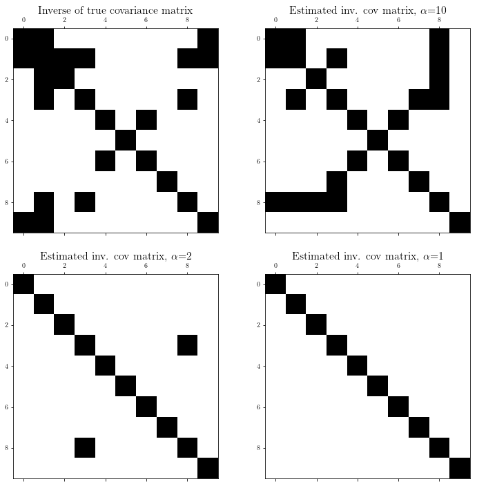
# Plot sparsity pattern for the true covariance matrix.
plt.subplot(2, 2, 1)
plt.spy(Strue)
plt.title('Inverse of true covariance matrix', fontsize=16)
# Plot sparsity pattern for each result, corresponding to a specific alpha.
for i in range(len(alphas)):
plt.subplot(2, 2, 2+i)
plt.spy(Ss[i])
plt.title('Estimated inv. cov matrix, $\\alpha$={}'.format(alphas[i]), fontsize=16)
<Figure size 432x288 with 0 Axes>