Fault detection¶

We’ll consider a problem of identifying faults that have occurred in a system based on sensor measurements of system performance.

Topic references¶

Samar, Sikandar, Dimitry Gorinevsky, and Stephen Boyd. “Likelihood Bounds for Constrained Estimation with Uncertainty.” Decision and Control, 2005 and 2005 European Control Conference. CDC-ECC’05. 44th IEEE Conference on. IEEE, 2005.

Problem statement¶

Each of \(n\) possible faults occurs independently with probability \(p\). The vector \(x \in \lbrace 0,1 \rbrace^{n}\) encodes the fault occurrences, with \(x_i = 1\) indicating that fault \(i\) has occurred. System performance is measured by \(m\) sensors. The sensor output is

\[\begin{equation} y = Ax + v = \sum_{i=1}^n a_i x_i + v, \end{equation}\]

where \(A \in \mathbf{R}^{m \times n}\) is the sensing matrix with column \(a_i\) being the fault signature of fault \(i\), and \(v \in \mathbf{R}^m\) is a noise vector where \(v_j\) is Gaussian with mean 0 and variance \(\sigma^2\).

The objective is to guess \(x\) (which faults have occurred) given \(y\) (sensor measurements).

We are interested in the setting where \(n > m\), that is, when we have more possible faults than measurements. In this setting, we can expect a good recovery when the vector \(x\) is sparse. This is the subject of compressed sensing.

Solution approach¶

To identify the faults, one reasonable approach is to choose \(x \in \lbrace 0,1 \rbrace^{n}\) to minimize the negative log-likelihood function

\[\begin{equation} \ell(x) = \frac{1}{2 \sigma^2} \|Ax-y\|_2^2 + \log(1/p-1)\mathbf{1}^T x + c. \end{equation}\]

However, this problem is nonconvex and NP-hard, due to the constraint that \(x\) must be Boolean.

To make this problem tractable, we can relax the Boolean constraints and instead constrain \(x_i \in [0,1]\).

The optimization problem

\[\begin{split}\begin{array}{ll} \mbox{minimize} & \|Ax-y\|_2^2 + 2 \sigma^2 \log(1/p-1)\mathbf{1}^T x\\ \mbox{subject to} & 0 \leq x_i \leq 1, \quad i=1, \ldots n \end{array}\end{split}\]

is convex. We’ll refer to the solution of the convex problem as the relaxed ML estimate.

By taking the relaxed ML estimate of \(x\) and rounding the entries to the nearest of 0 or 1, we recover a Boolean estimate of the fault occurrences.

Example¶

We’ll generate an example with \(n = 2000\) possible faults, \(m = 200\) measurements, and fault probability \(p = 0.01\). We’ll choose \(\sigma^2\) so that the signal-to-noise ratio is 5. That is,

\[\begin{equation} \sqrt{\frac{\mathbf{E}\|Ax \|^2_2}{\mathbf{E} \|v\|_2^2}} = 5. \end{equation}\]

import numpy as np
import matplotlib.pyplot as plt

np.random.seed(1)

n = 2000
m = 200
p = 0.01
snr = 5

sigma = np.sqrt(p*n/(snr**2))
A = np.random.randn(m,n)

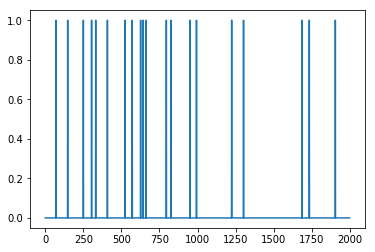
x_true = (np.random.rand(n) <= p).astype(int)
v = sigma*np.random.randn(m)

y = A.dot(x_true) + v

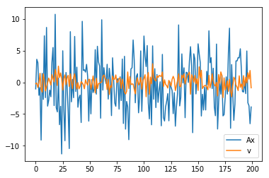
Below, we show \(x\), \(Ax\) and the noise \(v\).

plt.plot(range(n),x_true)

[<matplotlib.lines.Line2D at 0x11ae42518>]

plt.plot(range(m), A.dot(x_true),range(m),v)
plt.legend(('Ax','v'))

<matplotlib.legend.Legend at 0x11aee9630>

Recovery¶

We solve the relaxed maximum likelihood problem with CVXPY and then round the result to get a Boolean solution.

%%time
import cvxpy as cp
x = cp.Variable(shape=n)
tau = 2*cp.log(1/p - 1)*sigma**2
obj = cp.Minimize(cp.sum_squares(A*x - y) + tau*cp.sum(x))
const = [0 <= x, x <= 1]
cp.Problem(obj,const).solve(verbose=True)
print("final objective value: {}".format(obj.value))

# relaxed ML estimate
x_rml = np.array(x.value).flatten()

# rounded solution
x_rnd = (x_rml >= .5).astype(int)

ECOS 2.0.4 - (C) embotech GmbH, Zurich Switzerland, 2012-15. Web: www.embotech.com/ECOS

It     pcost       dcost      gap   pres   dres    k/t    mu     step   sigma     IR    |   BT
+7.343e+03  -3.862e+03  +5e+04  5e-01  5e-04  1e+00  1e+01    ---    ---    1  1  - |  -  -
+4.814e+02  -9.580e+02  +8e+03  1e-01  6e-05  2e-01  2e+00  0.8500  1e-02   1  2  2 |  0  0
-2.079e+02  -1.428e+03  +6e+03  1e-01  4e-05  8e-01  2e+00  0.7544  7e-01   2  2  2 |  0  0
-1.321e+02  -1.030e+03  +5e+03  8e-02  3e-05  7e-01  1e+00  0.3122  2e-01   2  2  2 |  0  0
-2.074e+02  -8.580e+02  +4e+03  6e-02  2e-05  6e-01  9e-01  0.7839  7e-01   2  2  2 |  0  0
-1.121e+02  -6.072e+02  +3e+03  5e-02  1e-05  5e-01  7e-01  0.3859  4e-01   2  3  3 |  0  0
-4.898e+01  -4.060e+02  +2e+03  3e-02  8e-06  3e-01  5e-01  0.5780  5e-01   2  2  2 |  0  0
+7.778e+01  -5.711e+01  +8e+02  1e-02  3e-06  1e-01  2e-01  0.9890  4e-01   2  3  2 |  0  0
+1.307e+02  +6.143e+01  +4e+02  6e-03  1e-06  6e-02  1e-01  0.5528  1e-01   3  3  3 |  0  0
+1.607e+02  +1.286e+02  +2e+02  3e-03  4e-07  3e-02  5e-02  0.8303  3e-01   3  3  3 |  0  0
+1.741e+02  +1.557e+02  +1e+02  2e-03  2e-07  2e-02  3e-02  0.6242  3e-01   3  3  3 |  0  0
+1.834e+02  +1.749e+02  +5e+01  8e-04  9e-08  8e-03  1e-02  0.8043  3e-01   3  3  3 |  0  0
+1.888e+02  +1.861e+02  +2e+01  3e-04  3e-08  2e-03  4e-03  0.9175  3e-01   3  3  2 |  0  0
+1.909e+02  +1.902e+02  +4e+00  7e-05  7e-09  6e-04  1e-03  0.8198  1e-01   3  3  3 |  0  0
+1.914e+02  +1.912e+02  +1e+00  2e-05  2e-09  2e-04  3e-04  0.8581  2e-01   3  2  3 |  0  0
+1.916e+02  +1.916e+02  +1e-01  2e-06  3e-10  2e-05  4e-05  0.9004  3e-02   3  3  3 |  0  0
+1.916e+02  +1.916e+02  +4e-02  7e-07  8e-11  7e-06  1e-05  0.8174  1e-01   3  3  3 |  0  0
+1.916e+02  +1.916e+02  +8e-03  1e-07  1e-11  1e-06  2e-06  0.8917  9e-02   3  2  2 |  0  0
+1.916e+02  +1.916e+02  +2e-03  4e-08  4e-12  4e-07  5e-07  0.8588  2e-01   3  3  3 |  0  0
+1.916e+02  +1.916e+02  +2e-04  3e-09  3e-13  3e-08  5e-08  0.9309  2e-02   3  2  2 |  0  0
+1.916e+02  +1.916e+02  +2e-05  4e-10  4e-14  4e-09  6e-09  0.8768  1e-02   4  2  2 |  0  0
+1.916e+02  +1.916e+02  +4e-06  6e-11  6e-15  6e-10  9e-10  0.9089  6e-02   4  2  2 |  0  0
+1.916e+02  +1.916e+02  +1e-06  2e-11  2e-15  2e-10  2e-10  0.8362  1e-01   2  1  1 |  0  0

OPTIMAL (within feastol=1.8e-11, reltol=5.1e-09, abstol=9.8e-07).
Runtime: 6.538894 seconds.

final objective value: 191.6347201927456
CPU times: user 6.51 s, sys: 291 ms, total: 6.8 s
Wall time: 7.5 s

Evaluation¶

We define a function for computing the estimation errors, and a function for plotting \(x\), the relaxed ML estimate, and the rounded solutions.

import matplotlib

def errors(x_true, x, threshold=.5):
    '''Return estimation errors.

    Return the true number of faults, the number of false positives, and the number of false negatives.
    '''
    n = len(x_true)
    k = sum(x_true)
    false_pos = sum(np.logical_and(x_true < threshold, x >= threshold))
    false_neg = sum(np.logical_and(x_true >= threshold, x < threshold))
    return (k, false_pos, false_neg)

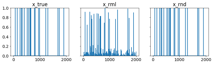
def plotXs(x_true, x_rml, x_rnd, filename=None):
    '''Plot true, relaxed ML, and rounded solutions.'''
    matplotlib.rcParams.update({'font.size': 14})
    xs = [x_true, x_rml, x_rnd]
    titles = ['x_true', 'x_rml', 'x_rnd']

    n = len(x_true)
    k = sum(x_true)

    fig, ax = plt.subplots(1, 3, sharex=True, sharey=True, figsize=(12, 3))

    for i,x in enumerate(xs):
            ax[i].plot(range(n), x)
            ax[i].set_title(titles[i])
            ax[i].set_ylim([0,1])

    if filename:
        fig.savefig(filename, bbox_inches='tight')

    return errors(x_true, x_rml,.5)

We see that out of 20 actual faults, the rounded solution gives perfect recovery with 0 false negatives and 0 false positives.

plotXs(x_true, x_rml, x_rnd, 'fault.pdf')

(20, 0, 0)